Diffusion Models

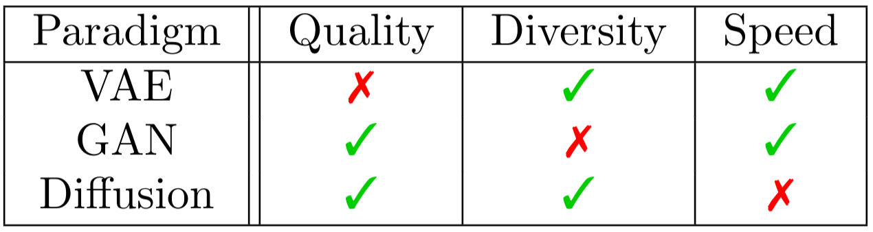
In this article I want to tell you about diffusion models, which is an actively developing approach to image generation. Recent research shows that this paradigm can generate images of quality on par with or even exceeding the one of the best GANs. Moreover, the design of such models allows them to surpass two main GANs’ weaknesses, i.e. mode collapsing and sensitivity to hyperparameter choice. However, the same design, that makes diffusion models so powerful, makes them considerably slower on inference.

Table taken from Aran Komatsuzaki’s blog post.

Diffusion models were first introduced in 2015 paper Deep Unsupervised Learning using Nonequilibrium Thermodynamics. The method goes as follows: we first define a Markovian noising process which gradually adds noise to objects from data distribution $x_0 \sim q(x_0)$ to produce noised samples $x_1, x_2, \ldots, x_T$, such that the last object $x_T$ comes approximately from standard normal distribution. If afterwards we can reverse this process, we can sample from the data distribution via sampling $x_T$ from standard normal distribution and applying our reversing procedure. If you’ve heard about the normalizing flows technique, than this might sound suspiciously familiar. However, in case of diffusion models we fix the forward trajectory of our process and obtain the reverse one by training our model to predict $x_{t-1}$ from $x_t$, as opposed to forcing our transformations to be inversible and training the forward trajectory.

That was the intuition, now let us look closely at a more formal definition of our model. As I already mentioned, we first need to define a Markov chain, that will take our source image $x_0$ and gradually add noise to it. Particularly, each step $t$ will add Gaussian noise according to some variance schedule $\beta_t$. However, simply adding noise isn’t enough, as we need to ensure that the mean value goes down to zero to comply with standard normal distribution. For this reason, before adding noise, we also multiply the object $x_{t-1}$ by $\sqrt{1 - \beta_t}$:

\[q(x_t \mid x_{t-1}) = \mathcal{N}(x_t \mid \sqrt{1 - \beta_t} x_{t-1},\ \beta_t \mathbf{I})\]

Authors note that, given each $\beta_t$ is small, we can view this process as continuos gaussian diffusion, which probably is the origin of the term diffusion models.

Here is how authors visualize the forward trajectory for a swiss roll data:

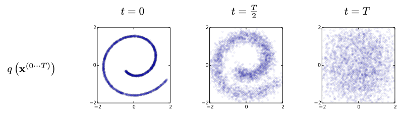
We start with a roll and gradually diffuse it step by step. In the middle of our chain we still can distinguish the spiral, but it is heavily blurred. If we then continue our diffusion, we’ll end up with a point cloud which looks a lot like a sample from a standard normal distribution.

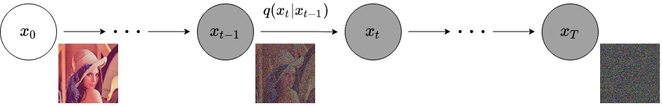
And this is how we can visualize the same process when working with images (visualization taken from another paper):

Authors note that schedule $\beta_t$ can be learned during training process, however this does not seem to provide any significant boost in quality. For this reason, authors stick with a pre-defined schedule and later articles tend to do so as well.

Defining the noising process in such a way has several important features. For example, there is no need to apply $q$ repeatedly to sample $x_t \sim q(x_t \mid x_0)$. Instead, we can derive $q(x_t \mid x_0)$ in closed form. If we denote

\[\alpha_t = 1 - \beta_t,\ \bar{\alpha}_t = \prod_{s=0}^t \alpha_s\]

we can show that:

\[q(x_t \mid x_0) = \mathcal{N}(x_t \mid \sqrt{\bar{\alpha}_t} x_0,\ (1 - \bar{\alpha}_t) \mathbf{I})\]

This is a very important formula and it has three important consequences.

The first one is the fact that, under reasonable settings for $\beta_t$ and $T$, distribution $q(x_T \mid x_0)$ is close to standard normal, just like we wanted.

The second consequence is the fact that we can rewrite that formula using the reparametrization trick:

\[x_t = \sqrt{\bar{\alpha}_t} x_0 + \sqrt{1 - \bar{\alpha}_t} \varepsilon,\ \varepsilon \sim \mathcal{N}(\varepsilon \mid 0,\ \mathbf{I})\]

This formula is the key to introducing the denosing diffusion probabilistic models and we will need it later on.

Last but not least, we can derive the posterior distribution $q(x_{t-1} \mid x_t, x_0)$ using Bayes theorem:

\[q(x_{t-1} \mid x_t, x_0) = \mathcal{N}(x_{t-1} \mid \tilde{\mu}(x_t, x_0),\ \tilde{\beta}_t \mathbf{I})\] \[\tilde{\mu}(x_t, x_0) = \frac{\sqrt{\bar{\alpha}_{t-1}} \beta_t}{1 - \bar{\alpha}_t} x_0 + \frac{\sqrt{\alpha_t} (1 - \bar{\alpha}_{t-1})}{1 - \bar{\alpha}_t} x_t\] \[\tilde{\beta}_t = \frac{1 - \bar{\alpha}_{t-1}}{1 - \bar{\alpha}_t} \beta_t\]

This formula is crucial to defining our loss later on, plus it gives the lower bound on the variance of the reverse step. Indeed, if we were to consider the entropy of the reverse step, we could constrain it from both sides. It turns out that the lower bound for the variance is given by $\tilde\beta_t$ (the minimum of variance is achieved when we know the true $x_0$) and the upper bound is given by $\beta_t$ (which is the actual amount of noise we add at the step $t$).

This concludes the forward trajectory. What about the reverse one? As I mentioned earlier, given $\beta_t$ is small, we can view our diffusion process as continuous, in which case reverse step $q(x_{t-1} \mid x_t)$ must have the identical functional form as the forward one. Since $q(x_t \mid x_{t-1})$ is a diagonal Gaussian distribution, then $q(x_{t-1} \mid x_t)$ should also be a diagonal Gaussian distribution meaning that on each step of the reverse trajectory we simply need to predict a mean $\mu_\theta(x_t, t)$ and a diagonal covariance matrix $\Sigma_\theta(x_t, t)$ in which case we would obtain:

\[p_\theta(x_{t-1} \mid x_t) = \mathcal{N}(x_{t-1} \mid \mu_\theta(x_t, t),\ \Sigma_\theta(x_t, t))\]

If now we found a way to train such model, we’d be able to reverse our diffusion process and convert our points from standard normal distribution back to points from data distribution $q(x_0)$.

Here is how it works with the swiss roll data:

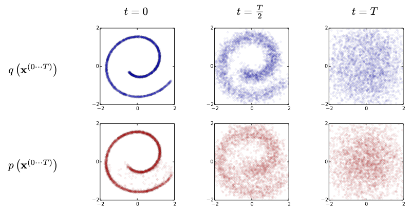
This time we go from right to left. We start of with a sample from standard normal distribution and gradually remove the noise from it. When we are half way through, we can see that the spiral starts to take form. At the end we see almost perfect roll.

Pretty much the same applies to images:

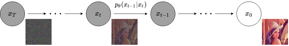
We start of with an image where each pixel value is sampled from standard normal distribution and gradually denoise it, until we reach the $x_0$ which should come approximately from empirical data distribution $q(x_0)$, i.e. should be an actual image.

At this point we know how to noise our images and how to reverse this process to restore our images. The only question left to answer is how do we train our model to correctly predict $\mu_\theta(x_t, t)$ and $\Sigma_\theta(x_t, t)$. Much like with most other probability-based approaches, we’d like to train our model via minimizing the negative log likelihood $\mathbb{E}[-\log p_\theta(x_0)]$. However, in this particular case, it may not be too easy: we don’t actually have the $p_\theta(x_0)$. What we have is a sequence of $p_\theta(x_{t-1} \mid x_t)$. We could multiply them together to obtain the joint distribution $p_\theta(x_0, \dots, x_T)$:

\[p_\theta(x_0, \dots, x_T) = p(x_T) \prod_{t=1}^T p_\theta(x_{t-1} \mid x_t)\]

However, we’d still need to take integral of it over all intermediate steps $x_1, \dots, x_T$ in order to get the required $p_\theta(x_0)$:

\[p_\theta(x_0) = \int p_\theta(x_0, \dots, x_T) dx_1 \dots dx_T\]

Unfortunately for us, this integral is not tractable, however, we can obtain a lower bound. First let’s multiply and divide the integral by $q(x_1, \dots, x_T \mid x_0)$:

\[p_\theta(x_0) = \int p_\theta(x_0, \dots, x_T) \frac{q(x_1, \dots, x_T \mid x_0)}{q(x_1, \dots, x_T \mid x_0)} dx_1 \dots dx_T =\] \[= \int q(x_1, \dots, x_T \mid x_0) \frac{p_\theta(x_0, \dots, x_T)}{q(x_1, \dots, x_T \mid x_0)} dx_1 \dots dx_T\]

This integral can be viewed as a mathematical expectation:

\[p_\theta(x_0) = \mathbb{E}_{q(x_1, \dots, x_T \mid x_0)} \left[ \frac{p_\theta(x_0, \dots, x_T)}{q(x_1, \dots, x_T \mid x_0)} \right]\]

If we now remember that we want to calculate the logarithm of likelihood, we could easily obtain a lower bound using the Jensen’s inequality:

\[\log p_\theta(x_0) = \log \mathbb{E}_{q(x_1, \dots, x_T \mid x_0)} \left[ \frac{p_\theta(x_0, \dots, x_T)}{q(x_1, \dots, x_T \mid x_0)} \right] \geq\] \[\geq \mathbb{E}_{q(x_1, \dots, x_T \mid x_0)} \left[ \log \frac{p_\theta(x_0, \dots, x_T)}{q(x_1, \dots, x_T \mid x_0)} \right] =\] \[= \int q(x_1, \dots, x_T \mid x_0) \log \frac{p_\theta(x_0, \dots, x_T)}{q(x_1, \dots, x_T \mid x_0)} dx_1 \dots dx_T\]

The last integral is here just as a reminder. After this equation I’ll just use the expectation form as it translates the same idea with less text. I’ll also shorten the base of expectation to just $q$ for the sake of cleaner formulae.

Now that we have our lower bound, let’s try and simplify it. First, let’s use the fact that both $p_\theta(x_0, \dots, x_T)$ and $q(x_1, \dots, x_T \mid x_0)$ are factorisable by our trajectory step:

\[\log p_\theta(x_0) \geq \mathbb{E}_q \left[ \log \frac{p_\theta(x_0, \dots, x_T)}{q(x_1, \dots, x_T \mid x_0)} \right] =\] \[= \mathbb{E}_q \left[ \log \left( p(x_T) \prod_{t=1}^T \frac{p_\theta(x_{t-1} \mid x_t)}{q(x_t \mid x_{t-1})} \right) \right]\]

We ended up with a logarithm of product, which equals to sum of logarithms:

\[\log p_\theta(x_0) \geq \mathbb{E}_q \left[ \log \left( p(x_T) \prod_{t=1}^T \frac{p_\theta(x_{t-1} \mid x_t)}{q(x_t \mid x_{t-1})} \right) \right] =\] \[= \mathbb{E}_q \left[ \log p(x_T) + \sum_{t=1}^T \log \frac{p_\theta(x_{t-1} \mid x_t)}{q(x_t \mid x_{t-1})} \right] =\] \[= \mathbb{E}_q \left[ \log p(x_T) + \sum_{t=2}^T \log \frac{p_\theta(x_{t-1} \mid x_t)}{q(x_t \mid x_{t-1})} + \log \frac{p_\theta(x_0 \mid x_1)}{q(x_1 \mid x_0)} \right]\]

Let’s leave the first and last terms as is and focus on the sum in the middle. As we agreed before, our forward trajectory $x_0, \dots, x_T$ is a Markov chain, hence $q(x_t \mid x_{t-1}) = q(x_t \mid x_{t-1}, x_0)$.

Also recall the Bayes theorem:

\[q(x_t \mid x_{t-1}, x_0) = \frac{q(x_{t-1} \mid x_t, x_0) q(x_t \mid x_0)}{q(x_{t-1} \mid x_0)}\]

If we substitute this to our sum, we will get the following:

\[\sum_{t=2}^T \log \frac{p_\theta(x_{t-1} \mid x_t)}{q(x_t \mid x_{t-1})} = \sum_{t=2}^T \log \left( \frac{p_\theta(x_{t-1} \mid x_t)}{q(x_{t-1} \mid x_t, x_0)} \cdot \frac{q(x_{t-1} \mid x_0)}{q(x_t \mid x_0)} \right) =\] \[= \sum_{t=2}^T \log \frac{p_\theta(x_{t-1} \mid x_t)}{q(x_{t-1} \mid x_t, x_0)} + \sum_{t=2}^T \log \frac{q(x_{t-1} \mid x_0)}{q(x_t \mid x_0)}\]

Once again, let’s leave the first group of terms as is and look a bit closer at the second sum:

\[\sum_{t=2}^T \log \frac{q(x_{t-1} \mid x_0)}{q(x_t \mid x_0)} = \sum_{t=2}^T (\log q(x_{t-1} \mid x_0) - \log q(x_t \mid x_0))\]

In this sum, each term contains the same component as the previous term, but with opposite sign. Hence, after summation, only two edge components will remain:

\[\sum_{t=2}^T \log \frac{q(x_{t-1} \mid x_0)}{q(x_t \mid x_0)} = \log q(x_1 \mid x_0) - \log q(x_T \mid x_0)\]

After substituting this into the previous formula we get:

\[\sum_{t=2}^T \log \frac{p_\theta(x_{t-1} \mid x_t)}{q(x_t \mid x_{t-1})} = \sum_{t=2}^T \log \frac{p_\theta(x_{t-1} \mid x_t)}{q(x_{t-1} \mid x_t, x_0)} + \log q(x_1 \mid x_0) - \log q(x_T \mid x_0)\]

And after substituting this into the log likelihood lower bound and merging $\log q(x_1 \mid x_0)$ with $\log \frac{p_\theta(x_0 \mid x_1)}{q(x_1 \mid x_0)}$ and $\log q(x_T \mid x_0)$ with $\log p(x_T)$ we obtain:

\[\log p_\theta(x_0) \geq \mathbb{E}_q \left[ \log p(x_T) + \sum_{t=2}^T \log \frac{p_\theta(x_{t-1} \mid x_t)}{q(x_t \mid x_{t-1})} + \log \frac{p_\theta(x_0 \mid x_1)}{q(x_1 \mid x_0)} \right] =\] \[= \mathbb{E}_q \left[ \log \frac{p(x_T)}{q(x_T \mid x_0)} + \sum_{t=2}^T \log \frac{p_\theta(x_{t-1} \mid x_t)}{q(x_{t-1} \mid x_t, x_0)} + \log p_\theta(x_0 \mid x_1) \right]\]

And the last step is to recognise the Kullback–Leibler divergencies in first two terms:

\[\log p_\theta(x_0) \geq \mathbb{E}_q \left[ \log \frac{p(x_T)}{q(x_T \mid x_0)} + \sum_{t=2}^T \log \frac{p_\theta(x_{t-1} \mid x_t)}{q(x_{t-1} \mid x_t, x_0)} + \log p_\theta(x_0 \mid x_1) \right] =\] \[= - D_{KL} (q(x_T \mid x_0) \mid p(x_T)) - \sum_{t=2}^T D_{KL} (q(x_{t-1} \mid x_t, x_0) \mid p_\theta(x_{t-1} \mid x_t)) + \log p_\theta(x_0 \mid x_1)\]

Now recall that instead of maximizing the log likelihood, we often talk about minimizing the negative log likelihood, meaning that our objective will have to be negated. Also the formula above gives the log likelihood for one object $x_0$. What we want to minimize is the $\mathbb{E}[-\log p_\theta(x_0)]$, where the expectation is taken over the $x_0 \sim q(x_0)$. In real life we often don’t know the $q(x_0)$. However, we have a sample of objects from $q(x_0)$ (i.e. our dataset) and hence we can approximate the expectation using the Monte Carlo method.

As such we obtain the $L_\text{vlb}$ loss ($\text{vlb}$ stands for variational lower bound):

\[\mathbb{E}[-\log p_\theta(x_0)] \leq L_{\text{vlb}} = L_0 + \sum_{t=1}^T L_t\] \[L_0 = -\log p_\theta(x_0 \mid x_1)\] \[L_{t-1} = D_{KL} (q(x_{t-1} \mid x_t, x_0) \mid p_\theta(x_{t-1} \mid x_t))\] \[L_T = D_{KL} (q(x_T \mid x_0) \mid p(x_T))\]

Note that it is easy to get intuition on what each term does. The $L_0$ forces our model to give as much probability as possible to the target picture at the end of the chain. Each of the $L_{t-1}$ forces the inverse process to follow the predefined route. Finally, the $L_T$ doesn’t depend on our trainable parameters $\theta$ and stands there to remind us that there is an unavoidable error caused by the fact that $q(x_T \mid x_0)$, although very close to $p(x_T)$ (standard normal distribution), never matches it exactly.

Another important thing to note is the fact that despite we see multiple Kullback–Leibler divergencies, we don’t need to take any integrals during training. All terms $L_t$ contain KL divergencies between two normal distributions, which means that each KL divergence becomes simply the MSE loss between distributions’ expectations, normed on their variances, plus a distance between their variances.

Now we can train our model! The training goes as follows: we pick an image $x_0$ from our dataset, compute the noised images $x_1, \dots, x_T$ and for each one of those we predict $\mu_\theta(x_t, t)$ and $\Sigma_\theta(x_t, t)$ with out model. Once we have done this, we compute the likelihood lower bound and use it as loss function.

This wraps up theory introduced in 2015 paper. Authors train their model on several datasets including MNIST and CIFAR-10 and show following samples:

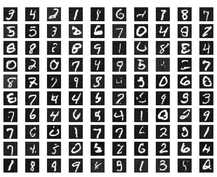
The samples might not look too appealing, but we have to cut authors some slack: first of all, it was back in 2015 and, second of all, authors used multi-layer perceptrons to predict $\mu_\theta(x_t, t)$ and $\Sigma_\theta(x_t, t)$ as opposed to using convolutional networks (remeber, 2015). The main contribution of this paper is the new approach, not an astonishing result.

Now we shall fast-forward to 2020 and look another paper called Denoising Diffusion Probabilistic Models (the name has became a term and is often reduced to DDPM). Authors of this work note that instead of predicting $\mu_\theta(x_t, t)$ and $\Sigma_\theta(x_t, t)$ it is benefitial to fix covariance to $\beta_t \mathbf{I}$ and predict the addendum noise $\varepsilon$ from the reparametrized equation

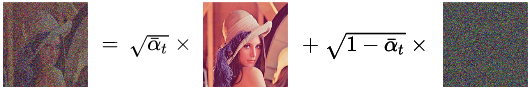
\[x_t = \sqrt{\bar{\alpha}_t} x_0 + \sqrt{1 - \bar{\alpha}_t} \varepsilon\]

instead of the $x_t$ itself. In this case instead of two models $\mu_\theta(x_t, t)$ and $\Sigma_\theta(x_t, t)$ we end up with just one model $\varepsilon_\theta(x_t, t)$.

Predicting random noise $\varepsilon_\theta(x_t, t)$ might seem odd at first. But let me be clear: the noise is random before we compute the $x_t$. Once we’ve computed the $x_t$, the $\varepsilon$ is fixed and our model needs to predict it via looking at the noised image $x_t$ and trying to decouple the noise from the original image $x_0$:

One advantage of such parametrization is the fact that now we don’t need to sample the whole forward trajectory $x_1, \dots, x_T$ in order to make a training step. We can just randomly pick a single step $t$ and we are good to go. In fact, we could do the same in previous model, but here it looks much more natural.

It is possible to train such model via minimizing the same objective $L_{\text{vlb}}$. As we’ve fixed covariances, KL divergencies would transform into MSE losses between the distribution expectancies divided by $\beta_t$. Due to our choice of parametrization, we can further simplify those to just the MSE losses between the predicted noises $\varepsilon_\theta(x_t, t)$ and the actual noises $\varepsilon$, once again divided by $\beta_t$. However, authors find that removing the division by $\beta_t$ actually improves the model performance. And this is how the simple objective was born:

\[L_{\text{simple}} = \mathbb{E}_{x_0 \sim q(x_0), t\sim[1, T], \varepsilon \sim \mathcal{N}(0, \mathbf{I})} [\| \varepsilon - \varepsilon_\theta(x_t, t) \|^2]\]

The training goes as follows: we choose an image $x_0$ from training dataset, sample step $t \sim \text{U}[0, T]$ and noise $\varepsilon \sim \mathcal{N}(0, \mathbf{I})$. We then compute $x_t$, predict $\varepsilon_\theta(x_t, t)$ and minimize MSE loss between it and the actual $\varepsilon$.

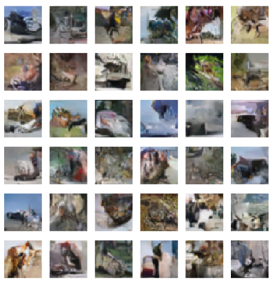
Apart from the noise prediction, authors also ditch the MLP and use a modern U-Net based convolutional architecture. They train their model on several datasets including CelebA-HQ, LSUN and CIFAR-10. Here is a sample from their models:

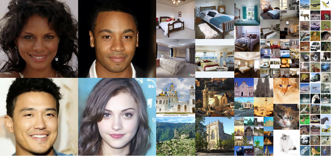
This looks much better! In fact, authors claim to have surpassed 2020 state-of-the-art FID score on CIFAR-10 dataset! However, CIFAR-10 is not that big of a dataset, especially for 2020 and I believe that this is not an accident. I believe that the size of dataset is exactly the problem that prevents a modern-sized GAN model to efficiently train. And this is diffusion models’ time to shine, as the fundamentally different, much more dense loss allows authors to train more sophisticated model on a smaller dataset without overfitting.

At this point we have a solid model which shows promissing results on smaller datasets, but cannot really compete with GANs on bigger ones. And this is where the OpenAI comes into play. OpenAI often plays a special role in ML community, as they have lots of computational power and they don’t hesitate to take existing models, scale them and write papers describing results they get. This happend with GPT-n models, R2D2 and, in 2021, the same happend with DDPM, when they published a paper called Diffusion Models Beat GANs on Image Synthesis. Here authors scaled the model plus introduced several improvements in order to beat GANs once and for all.

First of all, instead of fixing the variance $\Sigma_\theta(x_t, t)$ they use additional network to predict $v(x_t, t)$ and interpolate it between lower bound $\tilde\beta_t$ and upper bound $\beta_t$ in logarithmic scale:

\[\Sigma_\theta(x_t, t) = \exp(v(x_t, t) \log \beta_t + (1 - v(x_t, t)) \log \tilde\beta_t)\]

After this, authors can’t train the whole model with just simplified objective, as it doesn’t consider variance. In order to fix that authors use a hybrid objective $L_\text{simple} + \lambda L_\text{vlb}$.

Apart from that, authors propose several tricks in order to embed step number $t$ and class labels into their model. The first one of them is the use of adaptive group normalization. The second idea proposed in this article is the classifier guidance mechanism. Without going into much detail, idea here is to train a classifier on noised images $x_t$ and use its predictions to assert the target class, e.g. by adding gradient of log likelihood of the target class to $\mu_\theta(x_t, t)$.

All mentioned improvements allowed authors to achieve very convincing results on conditional ImageNet generation:

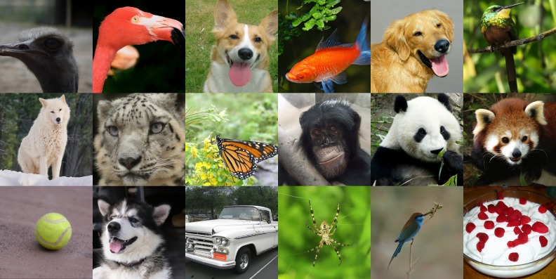
Additionaly, authors provide numerical evaluation of their models in terms of FID, sFID, precision and recall and compare their results with other models, both diffusion- and GAN-based. The model shows promissing results beating other models most of the time, while maintaining far superior coverage of the distribution modes.

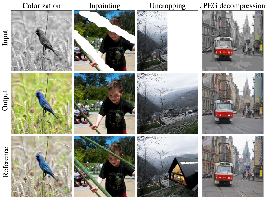
Last but not least, our journey cannot be completed until we talk about image-to-image generation. Indeed, natural generalization to image-to-image tasks is what made GANs so important to community. And so far it is not that obvious how to condition a diffusion model on, say, another image. And this is where Google Research comes into play. In their 2021 paper Palette: Image-to-Image Diffusion Models, authors say that it is sufficient to simply concatenate the conditioning image to the $x_t$ on each step (possibly upsampling the conditioning image in case of such tasks as super-resolution). Authors note that they’ve tried more sophisticated approaches, but the most obvious one shows the best results and can easily be generalized to basically any image-to-image generation task:

And thats it! This is basically all you need to know about diffusion models. Diffusion models showed themselves as a worthy competitor to GANs in terms of sample quality. Probably even to the extent where it is worth going straight for a DDPM instead of a GAN if quality is what you are looking for and the sampling speed is not crucial.

Right now there is an active research going on around DDPMs. Researchers are mostly focused on two main topics. The first one is finding even better architectures for DDPM networks in order to push the state-of-the-art in image generation. The second one is improving the sampling procedure in order to either speed up the sampling process or to be able to influence the sampling in a controled manner (which is closely related to the latent space exploration in GANs).

Anyways, those are mostly incremental improvements, which, I hope, you can easily understand after grasping this article. A good source of papers for further reading can be found here.